Sequential Testing for Experimental Design

Why Sequential Testing?

First, why should we do sequential testing? Why not just prespecify \(n\)?

Power Calculations

We can calculate the number of samples using a power calculation

(Boardwork)

Verify

library(pwr)
pwr.p.test(h = ES.h(0.15, 0.05), sig.level = 0.05, power = 0.90,
           alternative = "greater")


     proportion power calculation for binomial distribution (arcsine transformation) 

              h = 0.344372
              n = 72.21261
      sig.level = 0.05
          power = 0.9
    alternative = greater

Recall, using the SPRT we had on average less than 40 samples.

Always Do Sequential Testing Theorem

There is a theorem, which is hard to write down exactly, but I call it the Always Do Sequential Testing Theorem Wald (1945).

If you pick \(n\) via a power calculation, on average you could have gotten away with fewer samples had you used a sequential test instead.

Uses of Modern Sequential Testing

Platforms like Statsig implement the SPRT and it is quite easy to use.

AI Deployment Monitoring

Monitor model quality after deployment
Detect behaviors in real time without waiting for a fixed \(n\)
Training: Reinforcement Leanring as a type of experiment

Early Stopping for Clinical Trials

Stop early for efficacy or futility
FDA-recommended group sequential designs

From Testing to Confidence Sequences

There is a duality between Hypothesis Testing and Confidence Intervals
This same duality exists for sequential hypothesis testing

The SPRT requires the analyst to:

Know the distribution (and variance)
Specify the null and the alternative

We’ll introduce confidence sequences Waudby-Smith et al. (2024) — the sequential analogue of confidence intervals that remain valid at all sample sizes.

Simulation Setup

We consider a simple randomized experiment:

Parameter	Value	Description
\(n\)	1000	Total samples
\(p_0\)	0.4	Mean under control
\(p_1\)	0.6	Mean under treatment
\(e\)	0.5	Propensity score
\(\tau = p_1 - p_0\)	0.2	True ATE

The IPW estimator is \(\phi_i = \frac{Z_i Y_i}{e} - \frac{(1-Z_i)Y_i}{1-e}\)

`robbins_confseq` (click to expand)

Show robbins_confseq

library(ggplot2)
library(patchwork)

running_sd <- function(x) {
  n <- seq_along(x)
  M2 <- numeric(length(x))
  mu <- cumsum(x) / n
  for (t in 2:length(x)) {
    d <- x[t] - mu[t - 1]
    M2[t] <- M2[t - 1] + d * (x[t] - mu[t])
  }
  sqrt(pmax(M2 / pmax(n - 1, 1), 1e-10))
}

robbins_confseq <- function(x, alpha = 0.05, rho = 1) {
  n      <- seq_along(x)
  mu_hat <- cumsum(x) / n
  s_n    <- running_sd(x)
  radius <- s_n * sqrt((2 * (n * rho^2 + 1) / (n^2 * rho^2)) *
                         log(sqrt(n * rho^2 + 1) / alpha))
  data.frame(lower = mu_hat - radius, upper = mu_hat + radius)
}

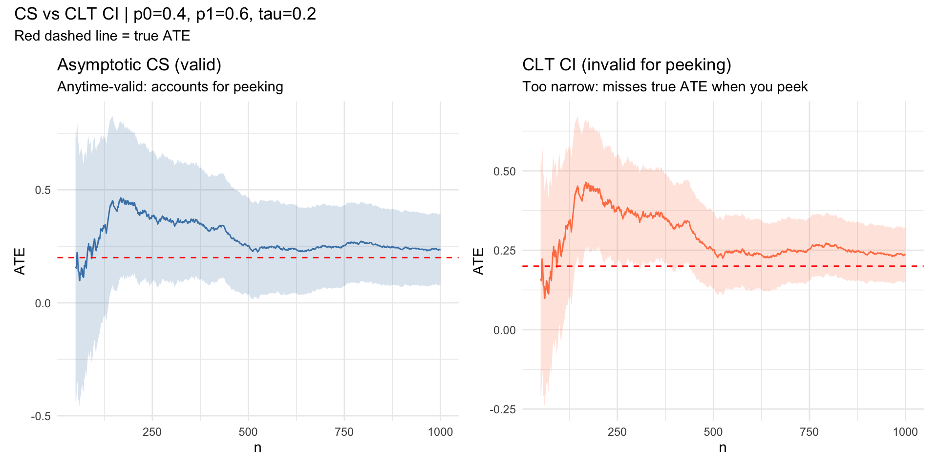
Confidence Sequences vs. CLT CI

Show simulation code

# --- Parameters ---
set.seed(7)
n <- 1e3; p0 <- 0.4; p1 <- 0.6; e <- 0.5
tau <- p1 - p0

Z   <- rbinom(n, 1, e)
Y   <- ifelse(Z == 1, rbinom(n, 1, p1), rbinom(n, 1, p0))
phi <- Z * Y / e - (1 - Z) * Y / (1 - e)

cs  <- robbins_confseq(phi)

ns     <- 1:n
mu_hat <- cumsum(phi) / ns
clt_hw <- qnorm(0.975) * running_sd(phi) / sqrt(ns)

df <- data.frame(
  t      = ns,
  ate    = mu_hat,
  cs_lo  = cs$lower, cs_hi = cs$upper,
  clt_lo = mu_hat - clt_hw,
  clt_hi = mu_hat + clt_hw
)[50:n, ]

p1_plot <- ggplot(df, aes(t)) +
  geom_ribbon(aes(ymin = cs_lo, ymax = cs_hi), alpha = 0.2, fill = "steelblue") +
  geom_line(aes(y = ate), color = "steelblue") +
  geom_hline(yintercept = tau, color = "red", linetype = "dashed") +
  labs(x = "n", y = "ATE", title = "Asymptotic CS (valid)",
       subtitle = "Anytime-valid: accounts for peeking") +
  theme_minimal()

p2_plot <- ggplot(df, aes(t)) +
  geom_ribbon(aes(ymin = clt_lo, ymax = clt_hi), alpha = 0.2, fill = "coral") +
  geom_line(aes(y = ate), color = "coral") +
  geom_hline(yintercept = tau, color = "red", linetype = "dashed") +
  labs(x = "n", y = "ATE", title = "CLT CI (invalid for peeking)",
       subtitle = "Too narrow: misses true ATE when you peek") +
  theme_minimal()

p1_plot + p2_plot +
  plot_annotation(
    title    = sprintf("CS vs CLT CI | p0=%.1f, p1=%.1f, tau=%.1f", p0, p1, tau),
    subtitle = "Red dashed line = true ATE"
  )

Artillery Example

Wald wanted a method that allowed him to stop monitoring the moment he could reject.
What if you were more flexible?

Group Sequential Designs

Instead of checking after every shell is fired
Let’s check at time 10, 20, 30, 40, 50
This is an example of a Group Sequential Design

Group Sequential Designs are Popular

FDA Guidance
Most popular method for A/B testers (Big tech)
They can visualized as a confidence sequence too.

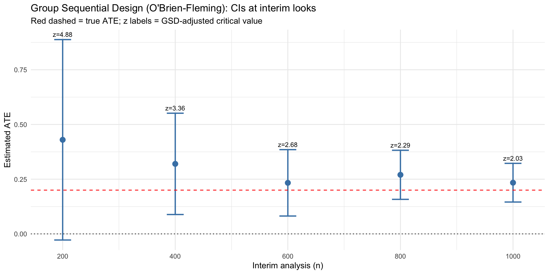
Group Sequential Designs in Action

References

Wald, A. 1945. “Sequential Tests of Statistical Hypotheses.” The Annals of Mathematical Statistics 16 (2): 117 186. https://doi.org/10.1214/aoms/1177731118.
Waudby-Smith, Ian, David Arbour, Ritwik Sinha, Edward H Kennedy, and Aaditya Ramdas. 2024. “Time-Uniform Central Limit Theory and Asymptotic Confidence Sequences.” The Annals of Statistics 52 (6): 26132640.