On Iterated Logarithms
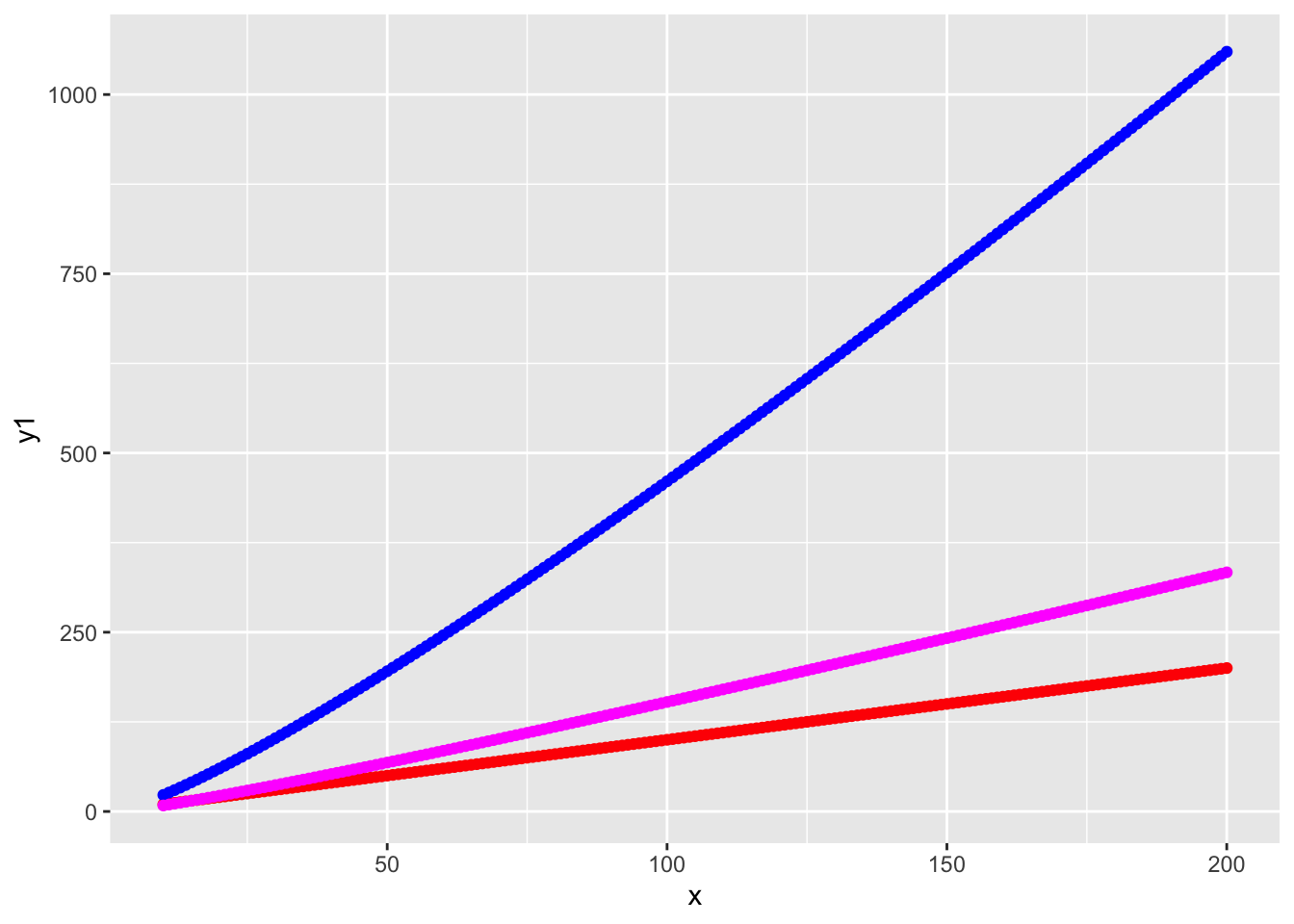
In undergraduate algorithms, you learn about algorithms to quickly sort your data. You learn for a list of \(n\) numbers you expect runtime to scale like \(O(n \log n)\). My professor told me that \(n\log n\) was nearly linear. If \(n \log n\) is nearly linear, then what is \(n \log (\log n)\)?
Looking at the plot, if \(n \log n\) is nearly linear, I’d be fine saying \(n \log \log n\) is linear.
Iterated logarithms are fun. For instance take some gigantic power like \(1000000 = k\). Then \[\log \log n^k \asymp \log \log n.\] The function is at a boundary of what is possible and what is not. Like the Erdös problems—they are not too hard but also not easy and eventually solvable. The function represents the edge of what is humanly possible and what is not. As made popular by the film Interstellar, Murphy’s law says “Whatever can happen will happen”.
I want to do some exposition on the role of iterated logarithms in Statistics. First, iterated logarithms usually conjure up an image of the Law of Iterated Logarithms (LIL). Most PhDs students haven taken a measure theory course know that it exists, but maybe not exactly what it is. They likely do not know that there are two LILs, with the more interesting one often referred to as the “other” LIL. In the popular Durrett textbook the LIL appears in the end where some classes fail to get to. In fact, I took both semesters of Measure theory at Duke (where Durrett is professor emeritus) and we never covered the law of iterated logarithm.
Second, the function showes up other places. These places are hard to find. If you type in “iterated logarithm {statistics, probability}” in Google or your favorite LLM, you’ll be flooded with the (main) LIL. So when you find a place the function shows up otherwise, you bookmark it. Here I’ll try to bookmark all of them and draw connections. Moreover, I want to investigate where the \(\pi\) comes from in the the “other” LIL.
But first we begin with the main LIL.
The (Main) Law of Iterated Logarithm
The usual motivation of the LIL is to consider two well known probabilistic laws: the Strong Law of Large Numbers (SLLN) and the Central Limit Theorem (CLT).
Let \(X_1, X_2, \sim \mathsf P\) independently where \(\mathsf P\) is any distribution with mean \(0\) and variance \(1\). Denote \(S_n = \sum_{i=1}^{n}X_i\). We have a spectrum from CLT to SLLN \[ \frac{S_n}{\sqrt{n}} \Rightarrow N(0,1), \quad \frac{S_n}{n} \to 0, \mathsf P-{\rm a.s.}. \] If we divide by square root \(n\) we get a weak convergence to a distribution. If we divide by something more powerful we lose all randomness and converge to a number.
The LIL asks what is a function \(f(n)\) that sits between these two functions: \(\sqrt{n} \lesssim f(n) \lesssim n\) where we don’t lose all randomness but we get an almost sure bound.
That function turns out to be \(f(n) = \sqrt{n \log \log n}\), and we obtain the LIL:
\[ \limsup_{n \to \infty} \frac{|S_n|}{\sqrt{2n \log \log n}} = 1, \mathsf P-{\rm a.s.}. \] This statement is oftentimes treated like a cool fact you can use in statistics trivial pursuit. Yet it pops up everywhere in sequential inference, which I will discuss next.