library(ggplot2)
library(patchwork)
# --- Parameters ---
n <- 1e3; p0 <- 0.4; p1 <- 0.6; e <- 0.5
tau <- p1 - p0
running_sd <- function(x) {
n <- seq_along(x)
M2 <- numeric(length(x))
mu <- cumsum(x) / n
for (t in 2:length(x)) {
d <- x[t] - mu[t - 1]
M2[t] <- M2[t - 1] + d * (x[t] - mu[t])
}
sqrt(pmax(M2 / pmax(n - 1, 1), 1e-10))
}
robbins_confseq <- function(x, alpha = 0.05, rho = 1) {
n <- seq_along(x)
mu_hat <- cumsum(x) / n
s_n <- running_sd(x)
radius <- s_n * sqrt((2 * (n * rho^2 + 1) / (n^2 * rho^2)) *
log(sqrt(n * rho^2 + 1) / alpha))
data.frame(lower = mu_hat - radius, upper = mu_hat + radius)
}
Z <- rbinom(n, 1, e)
Y <- ifelse(Z == 1, rbinom(n, 1, p1), rbinom(n, 1, p0))
phi <- Z * Y / e - (1 - Z) * Y / (1 - e)
cs <- robbins_confseq(phi)
ns <- 1:n
mu_hat <- cumsum(phi) / ns
clt_hw <- qnorm(0.975) * running_sd(phi) / sqrt(ns)
df <- data.frame(
t = ns,
ate = mu_hat,
cs_lo = cs$lower, cs_hi = cs$upper,
clt_lo = mu_hat - clt_hw,
clt_hi = mu_hat + clt_hw
)[50:n, ]
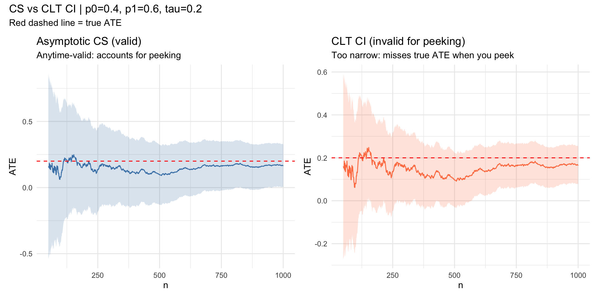
p1_plot <- ggplot(df, aes(t)) +
geom_ribbon(aes(ymin = cs_lo, ymax = cs_hi), alpha = 0.2, fill = "steelblue") +
geom_line(aes(y = ate), color = "steelblue") +
geom_hline(yintercept = tau, color = "red", linetype = "dashed") +
labs(x = "n", y = "ATE", title = "Asymptotic CS (valid)",
subtitle = "Anytime-valid: accounts for peeking") +
theme_minimal()
p2_plot <- ggplot(df, aes(t)) +
geom_ribbon(aes(ymin = clt_lo, ymax = clt_hi), alpha = 0.2, fill = "coral") +
geom_line(aes(y = ate), color = "coral") +
geom_hline(yintercept = tau, color = "red", linetype = "dashed") +
labs(x = "n", y = "ATE", title = "CLT CI (invalid for peeking)",
subtitle = "Too narrow: misses true ATE when you peek") +
theme_minimal()
p1_plot + p2_plot +
plot_annotation(
title = sprintf("CS vs CLT CI | p0=%.1f, p1=%.1f, tau=%.1f", p0, p1, tau),
subtitle = "Red dashed line = true ATE"
)